The brain is a complex system, and as all complex systems, its dynamics is highly nonlinear with complexity at many different scales. Large scale properties emerge from interactions at smaller scales but cannot be understood from the mechanisms of the smaller scales only. For example, at the molecular level one can study the mechanisms that generate action potentials in neurons but a perfect understanding of these mechanisms is not enough to understand how the brain is able to perform complex cognitive abilities such as memory, reasoning, spatial navigation, language, etc. Instead, the large scale of brain networks is more appropriate to gain insights on how the brain achieves such remarkable abilities. This is why it is important to model the dynamics of large networks of neurons.
The problem is that the brain contains millions of neurons and that it is impossible to simulate the dynamics at the level of single neuron when considering such a large number of them. Physics faced the same problem since it is impossible to solve the equations of motion for each of the \(10^{27}\) atoms of a gas. Statistical physics provides a procedure to go from a theory of the constituents at the microscale, to a macroscale description of the system. The main idea is to define macroscopic observables as statistical properties of the microstates of the system. For example the internal energy of a gas is defined as an average of the energy over all the microstates. A similar approach can be taken to study the dynamics of the brain at large scales. Indeed, large populations of neurons with similar properties can be found in the cortex and in such populations, one can simulate the mean firing activity of the population of neurons instead of the activity of individual neurons, which greatly reduces the computational cost.
In this blog post, I will present two such models, the rate model and the Wilson-Cowan model, and with the tools of the theory of nonlinear dynamical systems, we will analyse the dynamics of these models. Notably, we will see that the dynamics of the Wilson-Cowan model can exhibit hysteresis, limit cycles, and even a homoclinic orbit. At the end of this post, I provide a short list with some material on the subjects that I will talk about. The code used to make all the figures is available here and don’t hesitate to contact me by email if you have questions, remarks or if you want more details.
The rate model
The first model is a one-dimensional differential equation describing the dynamics of the mean activity of a population of neurons. This mean activity, also called firing rate or population activity, is denoted by \(A(t)\). Assuming that the population receives an external input \(I\) and that the neurons are not connected together, the rate model is the following
\[\tau \dfrac{dA}{dt} = -A + F(I)\]where \(\tau\) is a time constant and \(F\) is a nonlinear activation function relating the input of a neuron to its activity. The solution at equilibrium is defined by the equation \(\frac{dA}{dt}=0\), which simply gives \(A = F(I)\). Now, let’s consider a fully-connected population of neurons, with the same weight \(w\) for each connection. Then the rate model becomes
\[\tau \dfrac{dA}{dt} = -A + F(wA + I)\]The additional term \(wA\) inside \(F\) accounts for the inputs that each neuron receives from all the others. To found the equilibria, we can look at the solutions of the equation \(A = F(wA + I)\) but we have to be careful because the number of solutions depend on the form of the activation function \(F\) and on the external input \(I\). Let’s take a sigmoid activation function given by
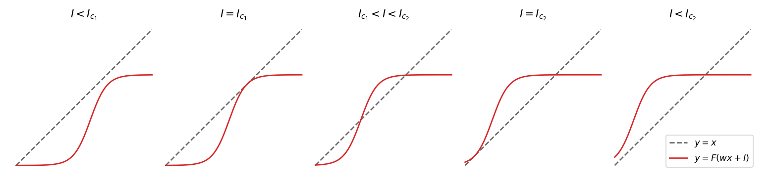
\[F(x) = \dfrac{1}{1+e^{-a(x-\theta)}} - \dfrac{1}{1+e^{a\theta}}\]where the parameter \(\theta\) is the position of the inflection point of the sigmoid, and \(\frac{a}{4}\) is the slope at \(\theta\). You can see the shape of this function in red on the plots just below. We will now study the equilibrium solutions as a function of the external input \(I\).
Saddle-node bifurcations and hysteresis
We can understand qualitatively how the solutions \(A = F(wA + I)\) vary with \(I\) by plotting the graphs \(y=x\) and \(y=F(wx+I)\) and looking at their intersections. The plots on the figure below show these graphs for different values of the external input \(I\). Let’s start with the leftmost plot, \(I\) is below a first critical threshold and there is only one equilibrium. Increasing \(I\) moves the graph of \(F\) towards the left, and at some point its upper part intersects with the line \(y=x\). There are now three equilibria. If \(I\) keeps increasing above a second critical threshold, the two lower equilibria disappear. So the behaviour of the system, i.e. towards which equilibrium state it will converge, depends critically on the value of \(I\). This abrupt change of behaviour when a parameter is changed is called a bifurcation of the system. For systems of dimensions less or equal to two, all the possible bifurcations can be classified. In this case, we have what is called two saddle-node bifurcations. We will encounter other types of bifurcations in the next section.
The next figure gives another visualisation of these saddle-node bifurcations. the x-axis is the external input \(I\) and the y-axis gives the equilibria of the system. We can see the two critical values of \(I\) (dotted lines) for which there is an abrupt change of behaviour. The stability of the equilibria is also represented with two stable equilibria (solid lines) and one unstable (dashed lines).
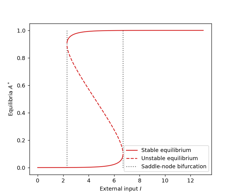
Even though this model is a crude approximation of the dynamics of real neurons in the brain, it can actually play the role of a short-term memory. To see this, let’s consider that the neural activity is initially at rest, i.e. \(A\) is small, and that the external input \(I\) is situated between the two critical thresholds (dotted lines on the figure above). An external stimulation will increase the value of \(I\) but the activity \(A\) will remained attracted to the stable equilibrium of low activity, until \(I\) crosses the second critical threshold. At this point the low activity equilibrium disappears and the state converges towards the only equilibrium remaining, which is an equilibrium of high neural activity. When the external stimulation ceases, \(I\) comes back to its initial value but the neurons remain highly activity, playing the role of a memory of the stimulation. So the current state of the system depends on its history. This phenomenon is also well-know in physics under the name of hysteresis.
The Wilson-Cowan model
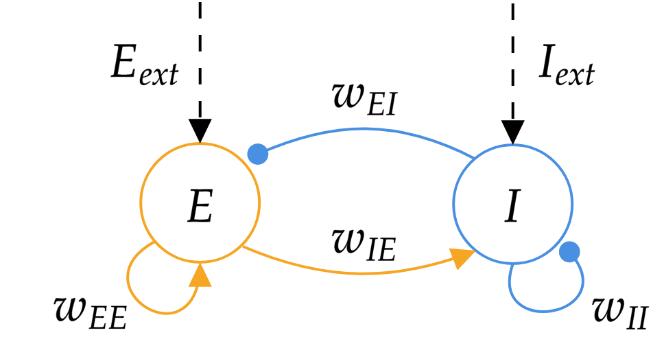
The second model that we will analyse is called the Wilson-Cowan model (original paper). This model also describes the dynamics of the mean activity but of two separate populations of neurons, one is excitatory and the other is inhibitory. The mean activity is denoted by \(E\) for the excitatory neurons, by \(I\) for the inhibitory neurons, and the dynamics for each population is taken to be the dynamics of the rate model described in the previous section. The two populations have recurrent connections and are connected to each other, as shown on the figure below. They also receive their own external input current, \(E_{ext}\) and \(I_{ext}\) for the \(E\) and \(I\) population, respectively.
We obtain the following coupled dynamical equations
\[\begin{aligned} \tau \dfrac{dE}{dt} &= -E + F(w_{EE}E - w_{EI}I + E_{ext})\\ \tau \dfrac{dI}{dt} &= -I + F(w_{IE}E - w_{II}I + I_{ext}) \end{aligned}\]where all the weights \(w_{EE}\), \(w_{EI}\), \(w_{IE}\), \(w_{II}\) are positive constants, and the inhibitory connections contribute negatively when summing the inputs of a population. The activation function \(F\) is the sigmoid function used in the previous section. The state space is two-dimensional, which allows for richer dynamics than the one-dimensional rate model as we will see in the subsequent sections.
Nullclines
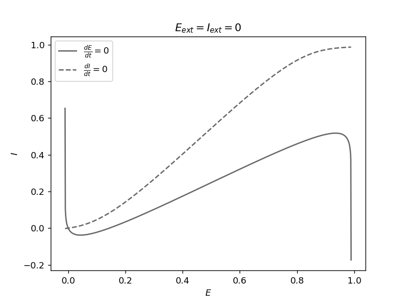
The equilibria of the system can be found by solving the equations \(\frac{dE}{dt}=0\) and \(\frac{dI}{dt}=0\), but these equations are often difficult to solve analytically for nonlinear dynamical systems. As in the previous section we can use a graphical method to understand qualitatively the solutions, and use numerical methods to obtain quantitative results. The equation \(\frac{dE}{dt}=0\) defines a curve in the \((E,I)\) plane which is called the E-nullcline, it is shown in solid line on the figure below. Similarly, \(\frac{dI}{dt}=0\) defines a curve called the I-nullcline and it is in dashed line on the figure. An equilibrium satisfies both of these equations and so it is an intersection of the E-nullcline and the I-nullcline. Note that while their intersections cannot be calculated directly, the equations of these nullclines can be obtained analytically and used to plot them. For the example of the figure below where the external inputs \(E_{ext}\) and \(I_{ext}\) are null, there is only one equilibrium corresponding to a state of low neural activity. We will use this graphical method again later on.
Stability and bifurcation diagram
Let’s try to understand the dynamical repertoire of the Wilson-Cowan model and in particular, what kind of dynamics can be found when varying the external inputs \(E_{ext}\) and \(I_{ext}\). More precisely, we would like to know the number and type of equilibria of the system for different values of the external inputs. The type of an equilibrium is determined by the eigenvalues of the system linearized around this equilibrium (see here for a characterization of the possible types of equilibrium in 2-dimension). The figure below shows this information for a regular grid of points in the \((E_{ext}, I_{ext})\) plane. For a particular point on this grid, the number of dots gives the number of equilibria, their shape represents their stability, and their color indicates whether their eigenvalues are real or complex conjugate.
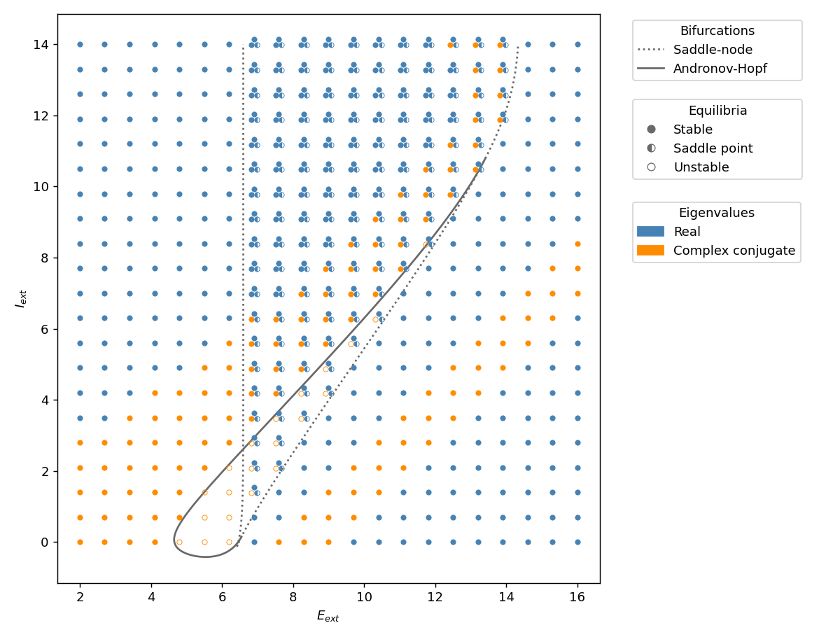
We can observe that the plane is partitioned into regions of similar behaviour and that there are curves separating those regions. Those curves are bifurcation curves and when they are crossed the number or stability of the equilibria changes abruptly. The solid line corresponds to a curve of so-called Hopf bifurcations and the dashed line is a curve of saddle-node bifurcations (the bifurcation that we encountered with the rate model). Note that those curves can be computed analytically but I will not detail the calculations here.
This diagram gives an overview of the dynamics of the Wilson-Cowan model and in the next sections, we will have a closer look at the behaviour of the system at different locations on this diagram. More specifically, we will see that the dynamics at the top of this diagram is very similar to the dynamics of the rate model. We will also encounter a region where the system produces oscillations. And finally, we will see what happens near a Bogdanov-Takens bifurcation point.
Hysteresis
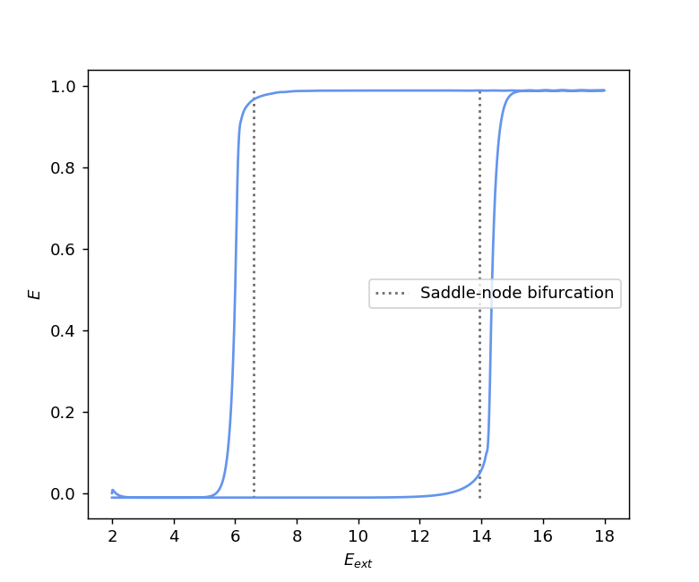
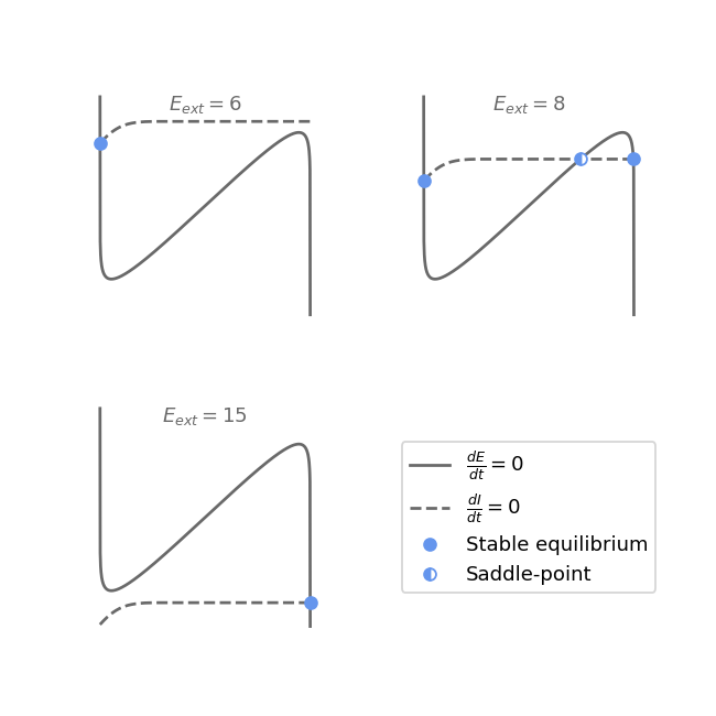
We can see on the diagram above that when \(I_{ext}\) is larger than more or less 11, the Hopf bifurcation curve stops, and there remains only the two saddle-node bifurcations. This situation is the same as in the rate model, and so we also have a hysteresis phenomenon here. Indeed, the first plot on the figure below shows a hysteresis for the excitatory activity \(E\) when \(E_{ext}\) varies. The external input \(E_{ext}\) is slowly increased and crosses the two saddle-node bifurcation curves before decreasing slowly back to its starting point, while \(I_{ext}\) is kept at a fixed value of 12. Note that we can observe a small discrepancy between the simulation (in solid line) and the theoretical bifurcations (in dotted lines), which is due to the incomplete relaxation to the equilibrium (in theory, the system needs an infinite amount of time to reach the equilibrium). The second part of the figure shows the nullclines as well as the equilibria of the system before, between, and after the two saddle-node bifurcations.
Limit cycle
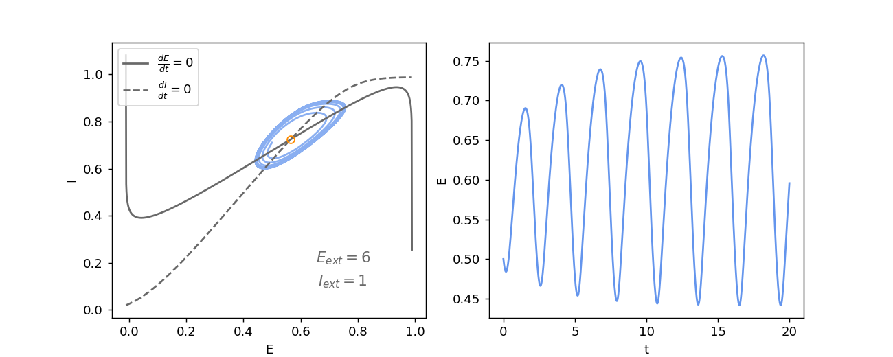
In the lower left part of the stability and bifurcation diagram, there is a region where the system has only one equilibrium whose type is an unstable focus (orange circle in the diagram). In such a case, there is a theorem, i.e. the Poincaré-Bendixson theorem, that proves that the state of the system converges to a periodic orbit. On the left of the figure below, we can see that the trajectory \((E(t), I(t))\) of the system is repelled from the equilibrium and that it converges towards a limit cycle. The right plot shows the oscillation of the activity of the excitatory population of the Wilson-Cowan model.
In the previous section, we saw a hysteresis for the activity of the excitatory population, which could play the role of a short-term memory. And here we have just seen that the exact same populations of neurons can also produce oscillations. The system can be moved from one dynamical regime to another by controlling the two external inputs of the populations. The flexibility of the behaviour of the Wilson-Cowan model is quite remarkable given the simplicity of this model.
Bogdanov-Takens bifurcation
We will see a last type of bifurcation which is a bit more advanced, so this last section is a bit more technical. Up to now the bifurcations that we encountered, i.e. the saddle-node and Hopf bifurcation, require only one parameter to be varied. The Bogdanov-Takens bifurcation requires two control parameters and it has a curve of saddle-node bifurcation, a curve of Hopf bifurcation, and a curve of homoclinic bifurcation. In the stability and bifurcation diagram, this bifurcation can be found at the intersections of the saddle-node and the Hopf bifurcation curves. If we go back to this diagram, the lowermost and the upper right intersections are Bogdanov-Takens bifurcations (the one around (6.5,3) is not because the Hopf bifurcation doesn’t involve the node of the saddle-node bifurcation).
Let’s analyse the upper right Bogdanov-Takens bifurcation, which is around (13.5, 11) in the diagram. After investigating a few simulations, we can determine that the Hopf bifurcation is subcritical, which consists in a stable focus absorbing an unstable limit cycle to become unstable. The homoclinic bifurcation curve is not represented in the diagram because it is difficult to compute it analytically. Nevertheless, with the knowledge of the Bogdanov-Takens bifurcation, we know that it is located just on the left of the subcritical Hopf bifurcation curve. The figure below shows some trajectories \((E(t), I(t))\) in the phase plane to better understand what happens in this Bogdanov-Takens bifurcation. Each color corresponds to an orbit whose starting point is denoted by a dot. The solid and dotted gray lines in the background are the E-nullcline and I-nullcline, respectively. The external input of the inhibitory population is kept fixed to \(I_{ext}=9\). While the external input \(E_{ext}\) starts on the left of the homoclinic bifurcation, and it will be increased so as to cross the homoclinic bifurcation first, the Hopf bifurcation second, and the saddle-node bifurcation last.
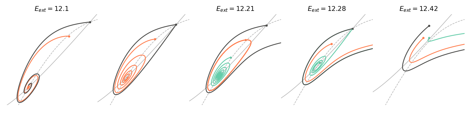
Let’s start with the leftmost plot of the figure above. There are two equilibria, a saddle-point and a stable focus (the third equilibrium, the stable node, is not of interest here). We can observe that the left unstable manifold of the saddle-point is attracted by the stable focus. Increasing a bit \(E_{ext}\) and we arrive at the homoclinic bifurcation. The homoclinic orbit is shown in black on the second plot, and it is unstable as the orange trajectory starting inside it converges towards the stable focus. Just after this bifurcation, an unstable limit cycle appears around the stable focus, depicted in orange on the third plot. Until the Hopf bifurcation, the unstable limit cycle shrinks, and finally, collapses on the focus. At this point, the focus loses its stability as it is observed on the fourth plot. The green trajectory spirals away from the node and, for this particular initial point, converges towards the stable manifold of the saddle-node. As the saddle-node bifurcation is crossed, the focus and the saddle-point collide and the two equilibria disappear. Finally, on the last plot, there is a saddle-node ghost that keeps influencing the trajectories.
Conclusion
We have seen that the Wilson-Cowan model has a rich dynamical repertoire. The system composed of a population of excitatory neurons and a population of inhibitory neurons can have quite different behaviour depending on the external inputs the populations receive. As in the case of the rate model, the neuronal activity can exhibit a hysteresis revealing a mechanism for short-term memory. The Wilson-Cowan model also explains how oscillations can be produced from excitation and inhibition, and it is kown that oscillations are omnipresent in the brain, often under the name of brain rythms. However their function is still not well understood. For example, they could organize the communication in the brain as the neuroscientist György Buzsáki wrote in his book The Brain from Inside Out (2019):
“the hierarchy of brain oscillations may parse and group neuronal activity to decompose and package neuronal information in communication between brain areas” (p.162)
Thus, this kind of model is a small step towards the understanding of the emergence of complex cognitive abilities from the dynamics of neurons.
Material
- Nonlinear Dynamics and Chaos (Strogatz, 2014) - an introductory book on the theory of nonlinear dynamical systems
- Excitatory and Inhibitory Interactions in Localized Populations of Model Neurons (Cowan, 1972) - the original paper of the Wilson-Cowan model
- Neuromatch Academy: Dynamic Networks - notebooks with exercices in python on the rate model and the Wilson-Cowan model
- Neuronal Dynamics (Gerstner, 2014) - a book with more advanced models of neurons and populations of neurons