The brain can be viewed as a computing or information processing machine where the relevant information is extracted from the sensory inputs. Similarly to our computers, the computations can be described as a sequence of instructions with algorithms. However, the brain is also very different from our computers and others prefer to view it as a dynamical system with continuous time dynamics at multiple temporal and spatial scales. How can we combine these two points of view ?

In this blog post, I will try to provide some intuition about how the dynamics of a neural network can compute something. As an example I will consider the Principal Component Analysis (PCA) method, which is a classical method for dimensionality reduction. The idea is to project high-dimensional data onto a smaller subspace in a way that captures as much as possible the relevant aspects of the data, and we will see what does that mean more precisely. After reviewing the basics of PCA, we will use a formulation of PCA as an optimization problem to build a continuous time dynamical system that computes this algorithm. The animation above hints the results obtained with the dynamical system that we will derive. We will see the importance of having two separate time scales for the dynamics and we will conclude that the principle used to build this simple example might be fundamental to better understand brain dynamics.

The code for this post can be found here and don’t hesitate to contact me by email if you have any questions or remarks.

Principal Component Analysis

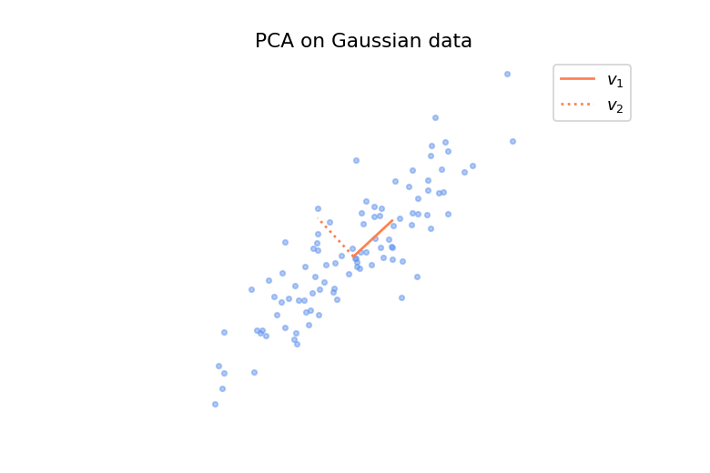
Let’s consider $m$ data points $\mathbf{x}^{(1)}, ..., \mathbf{x}^{(m)}$ in $\mathbb{R}^n$ drawn independently and identically (i.d.d.) from a distribution $p_{data}$, which is often called the data generating distribution. The PCA method assumes that the relevant directions are those along which the data vary the most, while those along which the data vary the least are considered as noise. It is important to note that this is an assumption and it will be satisfied or not depending on what your data represents and what you want to do with it. We can visualize more concretely what is a direction of maximal variance with a small example in $\mathbb{R}^2$. On the figure below is shown some data points sampled from a Gaussian distribution and we can see that there is a direction along which the data vary the most, depicted by the solid line segment.

The data $\mathbf{x}^{(1)}, ..., \mathbf{x}^{(m)}$ are assumed to be centered (zero mean) and let’s place them in a matrix $X$ such that the $i^{\text{th}}$ row is given by $(\mathbf{x}^{(i)})^T$. The goal of PCA is to find a subspace of dimension $r$ that captures as much variance as possible and to find an uncorrelated basis of this subspace. We will need the notion of the covariance matrix, so here is a short remark for those who are not familiar with it.

Remark: The covariance of two random variables $x_1$ and $x_2$ is defined as $\text{cov}(x_1, x_2) = \mathbb{E}[(x_1 - \mathbb{E}[x_1])(x_2 - \mathbb{E}[x_2])]$, which is equal to $\mathbb{E}[x_1x_2]$ if the variables have been centered beforehand so that they have zero mean. The entry at the $i^{\text{th}}$ row, $j^{\text{th}}$ column of the covariance matrix of a vector of random variables $\mathbf{x} = (x_1, ..., x_n)$ is given by $\text{cov}(x_i, x_j)$. The expectation over a random variable can be approximated by an average over data points sampled i.d.d. from its distribution. Thus, for centered data, $\text{cov}(x_i, x_j) \approx \frac{1}{m}\sum_{k=1}^m x_i^{(k)}x_j^{(k)}$ and the covariance matrix can be approximated by $\frac{1}{m}X^TX$. From now on, I will use this approximation but won’t make explicitly the distinction between random variable and data sample.

Let’s start by computing the singular value decomposition (SVD) $X = U\Sigma V^T$ where $U$ and $V$ are orthogonal matrices, and use it to define the following change of variable

This change of variable can be applied on each example $\mathbf{x}^{(i)}$ in $X$ to obtain a matrix $Y=XV$. Then using the fact that $X^TX = V\Sigma^2 V^T$, the covariance matrix of $\mathbf{y}$ is given by

Since $\Sigma$ is diagonal, this covariance matrix is diagonal. So we have $n$ uncorrelated random variables $y_i$ with respective variance given by the diagonal elements of $\Sigma^2$, i.e. $\text{var}(y_i) = \sigma_i^2$. From a geometrical point of view, the variable $y_i$ gives the component of the vector $\mathbf{x}$ projected onto the basis vector $\mathbf{v}_i$ which is the $i^{\text{th}}$ column of $V$. Hence, the direction of maximal variance is given by the vector $\mathbf{v}_1$ associated with the maximal singular value $\sigma_1$ (the singular values are ordered in decreasing order) and the corresponding variance is $\text{var}(y_1) = \sigma_1^2$. More generally, the subspace spanned by the $r$ first basis vectors $\mathbf{v}_1, ..., \mathbf{v}_r$ associated with the $r$ largest singular values $\sigma_1, ..., \sigma_r$ is the subspace of dimension $r$ that captures as much variance of the data as possible. Those $r$ basis vectors are called the $r$ first components of the data.

Optimization formulation

To build a dynamical system that computes the solution obtained above, it will be useful to express this solution as the solution of an optimization problem. Above we defined the vector $\mathbf{y}\in\mathbb{R}^n$ as $\mathbf{y}=V^T\mathbf{x}$, which contains the components of the orthogonal projection of the vector $\mathbf{x}$ onto the columns of $V$. As the goal is to compute the $r$-dimensional subspace of maximal variance, we are just interested in computing for each data point $\mathbf{x}$,

where $W \in \mathbb{R}^{n\times r}$ is the matrix containing the $r$ first columns of $V$, and $\mathbf{z} \in \mathbb{R}^r$ contains the components of the projection of $\mathbf{x}$ onto the columns of $W$. Now let’s show that this definition of $\mathbf{z}$ and $W$ is the solution of an optimization problem. To this end, we will use the following theorem.

Theorem (Low-rank approximation): The solution of

$$\min_{\hat{X}} ||\hat{X} - X||^2_F \quad \text{s.t. } \ \text{rank}(\hat{X}) \leq r$$

is $\hat{X} = \sigma_1 \mathbf{u}_1\mathbf{v}_1^T + ... + \sigma_r \mathbf{u}_r\mathbf{v}_r^T$, where $X = U\Sigma V^T$ is the SVD decomposition of $X$.

Let’s start with arbitrary $\mathbf{z}^{(i)}$ and matrix $W$ and let’s consider the minimization of the average reconstruction error between a data point $\mathbf{x}^{(i)}$ and the vector $W \mathbf{z}^{(i)}$,

where $\vert\vert\cdot\vert\vert_F$ is the Frobenius norm of a matrix, which can be written as the sum of the squared Euclidian norms of the rows of the matrix. The factor $\frac{1}{2}$ is just there to simplify the expression of the derivative. The matrix $\hat{X}$ contains the vectors $\mathbf{\hat{x}}^{(i)} = W \mathbf{z}^{(i)}$, $i = 1, ..., m$, in its rows and its rank is indeed lower or equal to $r$. Using the low-rank approximation theorem, the solution is

where $\equiv$ means that the equality holds by definition. From the fact that $W$ is constant for all data points and that it is $\mathbf{z}^{(i)}$ which depends on the input data $\mathbf{x}^{(i)}$, we can identify $z^{(i)}_j$ with $\sigma_j U_{ij}$ and the columns of $W$ with the vectors $\mathbf{v}_1, ..., \mathbf{v}_r$. Thus, we have obtained what we wanted for $W$, and actually for $\mathbf{z}$ too since

If we combine this result with the intuition from the previous section, projecting data points on the subspace of dimension $r$ which captures as much variance of the data as possible minimizes the average Euclidean norm of the reconstruction error. In this sense $\mathbf{z}$ is the best linear representation of dimension $r$ of the data. This is particularly useful when the data is high-dimensional since with $r \ll n$, we have a low-dimensional representation that can be useful to visualize the data for example.

Dynamical Equations

Now it’s time to derive the dynamical equations of a neural network computing PCA. We will need 3 groups of neurons: the input units for the input data $\mathbf{x}$, the internal units for the representation $\mathbf{z}$, and the output units for the reconstructed data $\mathbf{\hat{x}}$. As we will see, these neurons are connected together with weights given by the matrix $W$. Firstly, we need to specify the dynamics of the input units which represents the external input of the neural network. We will consider that a data point is drawn randomly from the data set and that it is presented to the neural network for a fixed amount of time $\tau$.

Fast dynamics

The output units compute a reconstruction $\mathbf{\hat{x}}$ of the input from the internal state $\mathbf{z}$ of the network, and the transformation is a linear one specified by the weights $W$. A simple dynamical model that achieves this is given by

since the equilibrium solution $\frac{d \mathbf{\hat{x}}}{dt}=0$ is $\mathbf{\hat{x}} = W \mathbf{z}$. The time constant $\tau_{fast}$ controls the rate of convergence towards the equilibrium. Next, to obtain the dynamical equations for $\mathbf{z}$ and $W$, we will use the optimization formulation of the previous section together with the following theorem.

Theorem: If a dynamical system can be written as $\frac{d\mathbf{x}}{dt} = - \nabla V(\mathbf{x})$ then

$$\frac{dV}{dt}(\mathbf{x}(t)) = \nabla V(\mathbf{x}(t)) \cdot \frac{d\mathbf{x}}{dt}(t) = -||\nabla V(\mathbf{x}(t))||^2 \leq 0$$

and $\frac{dV}{dt} = 0$ if and only if $\nabla V = 0$.

The function $V$ can only decrease on the trajectories of the system and the state converges towards a minimum of $V$. This is the equivalent of the gradient descent algorithm but in continuous time. If we take $V$ to be the objective that we are trying to minimize to compute the solution of PCA, its derivatives give us dynamical equations for $\mathbf{z}$ and $W$.

Let’s denote by $\mathbf{x}^{(i)}$ the current input. We would like the internal units $\mathbf{z}^{(i)}$ to compute the orthogonal projection of the input onto the columns of $W$, as it is the case in PCA. But we have to be careful because here we have a dynamical system where the units and the weights co-evolve, that is the weights $W$ are dynamically learned while the internal representation $\mathbf{z}^{(i)}$ is dynamically computed. Thus, the columns of $W$ will not be necessarily orthonormal especially if the weights are initialized randomly, and the projection cannot be computed as we did before . If we take the gradient with respect to $\mathbf{z}^{(i)}$of the reconstruction error $R$ defined in (1) and set it to zero, we obtain

which is the correct formula for the orthogonal projection on non orthonormal vectors (if $W^TW=I$ we recover $\mathbf{z}^{(i)} = W^T\mathbf{x}^{(i)}$). Using the theorem above, the following dynamics for the internal units will decrease the reconstruction error

And the time scale of the dynamics should be faster than the time scale of the input units, i.e. $\tau_{fast} \ll \tau$, so that the network has the time to compute the projection of the current input before it changes. Note that theoretically it requires an infinite amount of time to reach exactly the equilibrium but here we are only interested in an approximate solution and so being close to it is enough.

Slow dynamics

It remains to determine the dynamics of the weights. Similarly to what we did with the internal units, we can take the derivative of the reconstruction error with respect to $W$,

and use it to obtain a dynamical equation that would change the weights so as to minimize the reconstruction error, and so approximating PCA. The difference here is that we have a sum over the data points in the gradient which is problematic because only one data point at a time is shown to the network. The trick is to simply replace this sample average by a time average of the gradient evaluated at one data point sampled randomly. This is achieved by setting the time scale of the dynamics of the weights to a value much larger than the time scale at which the input data $\mathbf{x}$ is changed. Thus, we get the following dynamical equation

where $\tau \ll \tau_{slow}$. This trick is actually well-known in machine learning as it is very similar to stochastic gradient descent where the expectation of the gradient is replaced by the gradient evaluated at one data point sampled randomly from the data set. The slow time scale would then correspond to a small learning rate. The slow dynamics of the weights make them sensitive to the data distribution instead of the details of individual data points. This means that the weights capture the statistical regularities, the patterns in the activity of the neurons. The dynamical equation above is an example of a Hebbian learning rule where the weights change according to the correlation between the activity of the neurons they connect.

Fast and slow dynamics

To sum up, the dynamical equations of our network are

and $\mathbf{x}$ is sampled randomly from the data set at intervals $\tau$, with $\tau_{fast} \ll \tau \ll \tau_{slow}$. The following diagram illustrates the interactions between the different units of the network.

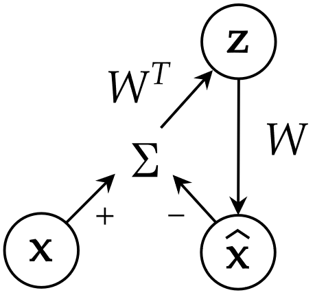
The important insight to remember from the derivation of these equations is that the dynamics of the internal state and the dynamics of the weights are governed by the same objective function, the difference resides in their respective time scale.

Simulations

Gaussian data

Let’s come back to the animation at the beginning of this post which is a visualization of our dynamical system computing PCA for Gaussian data in $\mathbb{R}^2$. The blue dots represent the whole data set, while the black dot corresponds to the input data that is currently presented to the network. The cross shows the reconstructed data obtained from the projection of $\mathbf{x}$ onto the vector $W$. The two vectors $\mathbf{v}_1$ and $\mathbf{v}_2$ in gray just indicate the two first components of the data. Note that I have not given any theoretical results on how to choose the time scales $\tau_{fast}$, $\tau$, and $\tau_{slow}$. What we can do is to inspect visually the dynamics of the system and see if it has the expected behaviour. For example on the left of the figure below, it seems that the slow time scale $\tau_{slow}$ is too fast as individual data points have a quite big influence on the weights. The example on the right seems to be better.

Fast and slow dynamics approximating PCA on Gaussian data

MNIST

Now, let’s see how it performs on images of digits. We will consider images of zero and one taken from the MNIST dataset. Each image has 28x28 pixels and so the input vector $\mathbf{x}$ lies in a space of dimension 784, which is much greater than the 2 dimensions in the example above. It is not possible to visualize directly what is happening in this high-dimensional space, instead what we can do is to project the whole space on the two first components $\mathbf{v}_1$, $\mathbf{v}_2$ of the data set, computed with the SVD decomposition of $X$. It gives us a window through which we can look at the high-dimensional dynamics and it allows us to see how close the columns $\mathbf{w_1}$and $\mathbf{w}_2$ of $W$ are to $\mathbf{v}_1$ and $\mathbf{v}_2$. If you look at the plots below, you will see that the vectors $\mathbf{v}_1$, $\mathbf{v}_2$ are shown in gray and in orange is shown the projections of $\mathbf{w}_1$, $\mathbf{w}_2$ onto the subspace spanned by these two vectors. If a projected orange segment has exactly the same length than the segments in gray, it means that the corresponding vector $\mathbf{w}$ belongs to the subspace spanned by $\mathbf{v}_1$, $\mathbf{v}_2$ and the longer its length, the more aligned it is with it.

The animation on the left shows the first 500 steps of a simulation of 4000 iterations, and the one on the right shows the last 500 steps. We can observe that at the beginning, the columns of $W$ which are initialized randomly are not at all aligned with the two first components, and so the internal representation $\mathbf{z}$ is not informative at all. As the network sees more and more images of digits, the weights learn to capture the statistical regularities in the data and at the end, the internal representation extracts meaningful information which allows us to distinguish the two digits. We can observe this on the animation on the right where the cross is correctly on the right for images of one and on the left for images of zero. However, it seems that the weights have more difficulties to capture the second component $\mathbf{v}_2$ of the data.

Fast and slow dynamics approximating PCA on MNIST

Conclusion

The goal of this post was not the provide rigorous results about convergence, uniqueness, etc, but to provide some intuition on how the dynamics of a neural network can approximately compute an algorithm. Even though the computation that our dynamical system realizes is way simpler than the computations that the brain realizes, the principle behind it might be fundamental to understand brain dynamics. It is the idea that the multi-scale dynamics is optimizing one objective function which is some kind of measure of the prediction error between inputs and predictions computed from internal representations. This is the idea of predictive coding or more generally, of the free energy principle where action, perception and learning are governed by the same objective function. In this framework, the fast dynamics of the internal units of our network is called perception and the slow dynamics of the weights, learning.